How to customize your own parallel
Define your own parallel model with LiBai.layers
Large-scale FC
Suppose you have a huge fully-connected-layer for large-scale classification (e.g., 1000w classes), which makes it impossible to fit into a single GPU.
Don’t worry, with the help of LiBai.layers, you can write models in a familiar way that you used to write models for a single GPU. We give a simple example showing how to write a tensor-parallel fully-connected-layer with 2 GPUs.
# huge_fc_example.py
import oneflow as flow
from omegaconf import DictConfig
from oneflow import nn

from libai.layers import Linear
from libai.utils import distributed as dist

cfg = DictConfig(dict(data_parallel_size=1, tensor_parallel_size=2, pipeline_parallel_size=1))
dist.setup_dist_util(cfg)


class Huge_FC(nn.Module):
    def __init__(self):
        super().__init__()
        self.fc = Linear(2048, 32768, parallel="col")

    def forward(self, x):
        return self.fc(x)


huge_fc = Huge_FC()

x = flow.rand(32, 2048, sbp=flow.sbp.broadcast, placement=flow.placement("cuda", ranks=[0, 1]))
y = huge_fc(x)

print(f"rank: {flow.env.get_rank()}, tensor shape: {y.to_local().shape}")
You can run this toy example with command line as follows:
python3 -m oneflow.distributed.launch --nproc_per_node 2 huge_fc_example.py

>> rank: 0, tensor shape: oneflow.Size([32, 16384])
>> rank: 1, tensor shape: oneflow.Size([32, 16384])
Through the result, you can find that y has been split along with axis=1 on 2 GPUs.
Large MLP models
Assume we have a huge MLP model which is very popular in transformer-based models, with a huge hidden size that makes it difficult to fit into a single GPU.
We can then split the model weights across GPUs in a hybrid parallel mode while you still write your model in a familiar way.
We give a simple example about the 2D parallel MLP in the LiBai context.
import oneflow as flow
from omegaconf import DictConfig
from oneflow import nn

from libai.layers import Linear
from libai.utils import distributed as dist

cfg = DictConfig(dict(data_parallel_size=2, tensor_parallel_size=2, pipeline_parallel_size=1))
dist.setup_dist_util(cfg)

# Write a Simple 2D Parallel MLP
class MLP_2D(nn.Module):
    def __init__(self):
        super().__init__()
        self.linear_1 = Linear(in_features=1024, out_features=16384, parallel="col")
        self.relu = nn.GELU()
        self.linear_2 = Linear(in_features=16384, out_features=1024, parallel="row")

    def forward(self, x):
        x = self.linear_1(x)
        x = self.relu(x)
        x = self.linear_2(x)
        return x

# define a model
mlp = MLP_2D()

# define input with 2D sbp
x = flow.rand(
    32,
    1024,
    sbp=dist.get_nd_sbp([flow.sbp.split(0), flow.sbp.broadcast]),
    placement=dist.get_layer_placement(0)
)
y = mlp(x)

print(f"rank: {flow.env.get_rank()}, tensor shape: {y.to_local().shape}")
You can run it with command line as follows:
python3 -m oneflow.distributed.launch --nproc_per_node 4 huge_mlp_example.py

>> rank: 2, tensor shape: oneflow.Size([16, 1024])
>> rank: 3, tensor shape: oneflow.Size([16, 1024])
>> rank: 1, tensor shape: oneflow.Size([16, 1024])
>> rank: 0, tensor shape: oneflow.Size([16, 1024])
From above, you can see that data are split into 2 groups for data parallel and weights are split into 2 groups for tensor model parallel. So this simple example just implements a 2D parallel.
For the sake of your convenience, we provide some prevalent models such as BERT, GPT-2, and ViT in Mode Zoo. Feel free to customize them into different sizes to fit into your special needs.
Write your own pipeline parallel model
In this tutorial, you will learn how to use pipeline parallel in your own model. In LiBai, we have two pipeline-parallel modes: naive pipeline parallel and (similar) 1F1B pipeline parallel introduced by Megatron-LM.
Introduction of naive pipeline parallel
In LiBai, naive pipeline parallel can be implemented by setting layers and parameters placement.
You can easily configure their placement by dist.get_layer_placement(idx).
We give an example for placement configuration.
# set a free tensor placement to first stage
self.pos_embed = nn.Parameter(
    flow.zeros(
        1,
        num_patches + 1,
        embed_dim,
        sbp=dist.get_nd_sbp([flow.sbp.broadcast, flow.sbp.broadcast]),
        placement=dist.get_layer_placement(0),
    )
)

# set a Linear placement to last stage
# set it manually
self.head = Linear(embed_dim, num_classes, layer_idx=-1).to_global(placement=dist.get_layer_placement(-1))
# use `layer_idx` API
self.head = Linear(embed_dim, num_classes, layer_idx=-1)
After configuring models placement, you need to add the input placement transition across different stages. In LiBai, we set a layer_idx attribute in each nn.Module, so you can simply add to_global in forward to implement input placement transition.
class MyModule(nn.Module):
    def __init__(self, ... *, layer_idx):
        ...
        self.layer_idx = layer_idx
        ...

    def forward(self, hidden_states):
        hidden_states = hidden_states.to_global(placement=dist.get_layer_placement(self.layer_idx))
        ...
After configuring models and data placement, the only thing that needs to do is setting the distributed configuration.
# set pipeline stages to 2
train.dist.pipeline_parallel_size = 2

# set model layers for pipeline
train.dist.pipeline_num_layers = hidden_layers
Introduction of 1F1B pipeline parallel
First of all, we will introduce GPipe to you for your better understanding. In GPipe, when the forward passes of all microbatches finish, the backward passes would be executed (shown in below).
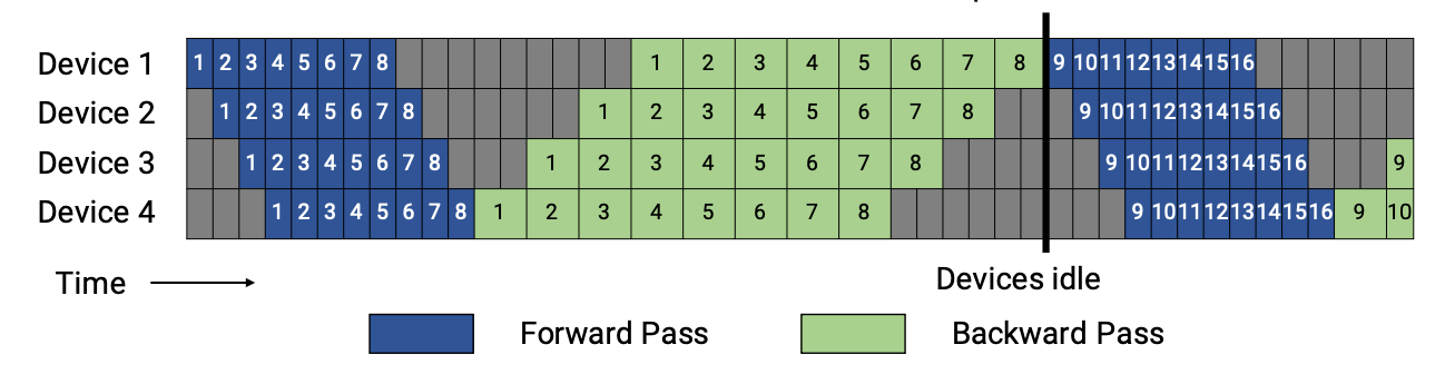
1F1B performs one forward pass followed by one backward pass. Finally, at the end of a batch, complete backward passes for all remaining in-flight microbatches. In general, 1F1B is more efficient than GPipe.
There are two schedules of 1F1B pipeline, the non-interleaved and the interleaved. The figures are shown below.
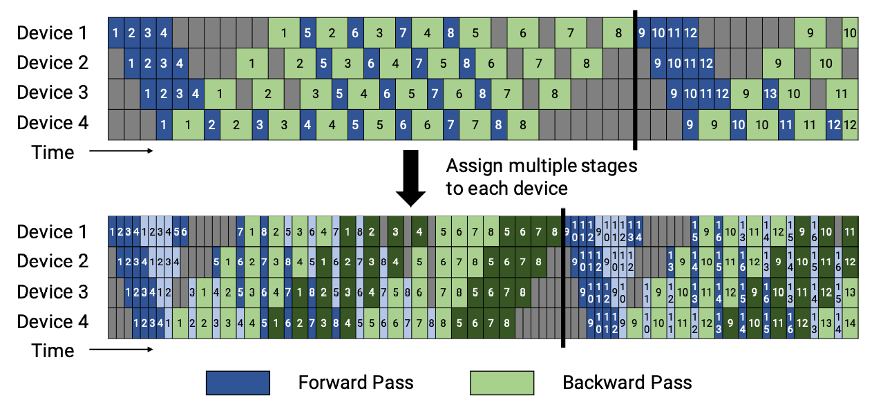
In LiBai, the non-interleaved schedule is supported currently, and this mode is more memory-efficient than GPipe.
The only thing that need to do is setting models stage id except that placement configuration in naive pipeline parallel, and stage id can help create stashed buffers for activation.
We will show you how to configure bert model stage id as an example.
class BertForPreTraining(nn.Module):
    def __init__(self, ...):
        ...
    def forward(self, ...):
        ...

    @staticmethod
    def set_pipeline_stage_id(model):
        dist_utils = dist.get_dist_util()

        # Set pipeline parallelism stage_id
        for module_block in model.modules():
            # module.origin can get the original module
            if isinstance(module_block.origin, BertEmbeddings):
                module_block.config.stage_id = dist_utils.get_layer_stage_id(0)
            elif isinstance(module_block.origin, BertExtendedAttnMask):
                module_block.config.stage_id = dist_utils.get_layer_stage_id(0)
            elif isinstance(module_block.origin, TransformerLayer):
                module_block.config.stage_id = dist_utils.get_layer_stage_id(module_block.layer_idx)
            elif isinstance(module_block.origin, BertPooler):
                module_block.config.stage_id = dist_utils.get_layer_stage_id(-1)
            elif isinstance(module_block.origin, BertPreTrainingHeads):
                module_block.config.stage_id = dist_utils.get_layer_stage_id(-1)

        # Set the last layernorm stage id
        model.bert.final_layernorm.config.stage_id = dist_utils.get_layer_stage_id(-1)
In set_pipeline_stage_id, BertEmbeddings and BertExtendedAttnMask are placed in the first stage, then each TransformerLayer is uniformly placed in each stages. At last, place BertPooler and BertPreTrainingHeads in the last stage. But don’t forget to place the last layernorm in BertEncoder which not belonging to any TransformerLayer to the last stage.
After adding the set_pipeline_stage_id function in a pre-defined nn.Module, GraphBase will invoke it automatically as below.
def set_pipeline_stage_id(self):
    if hasattr(type(self.model.origin), "set_pipeline_stage_id"):
        type(self.model.origin).set_pipeline_stage_id(self.model)
The last thing left is to set the training configuration as below
# set pipeline stages to 2
train.dist.pipeline_parallel_size = 2

# set model layers for pipeline
train.dist.pipeline_num_layers = hidden_layers

# enable activation checkpointing
train.activation_checkpoint.enabled = True

# enable gradient accumulation with 8 micro-batches
train.num_accumulation_steps = 8